
What GDP Can and Cannot Tell Us
By: Niaoniao You, EBRC Senior Economic Forecaster
Understanding GDP: Part 1 – How GDP is measured at national and regional levels
Gross Domestic Product, or GDP, is one of the most comprehensive measures of economic activity. It is defined as the total market value of all final goods and services produced within a region over a specific period, but what does that mean? And what can and can’t it tell us, at different geographic levels?
GDP is a definitive measure of the size and growth of economic activity, but it does not always tell us much about labor market conditions. In past decades, a slowdown in employment growth has mostly gone hand in hand with a slowdown in GDP. Exhibit 1 shows that U.S. real GDP annual growth generally moves together with the total nonfarm payroll job growth. Over the last few years, however, job growth has begun to decelerate, while real GDP growth has remained steady, boosting labor productivity (output per labor hour) mechanically.
Exhibit 1: Growth in U.S. Real GDP and Nonfarm Payroll Jobs, Over the Year, Percent
Previously, such divergence was typically observed during recoveries from recessions. From 2001 to 2003, GDP growth rebounded while nonfarm payroll jobs continued to decline after the 2001 recession. Economists attributed the productivity gains during that period to IT adoption. For the current productivity boost, while generative AI is a plausible factor, alternative factors, such as wider adoption of machine learning and flexibility in work arrangements, probably contributed.
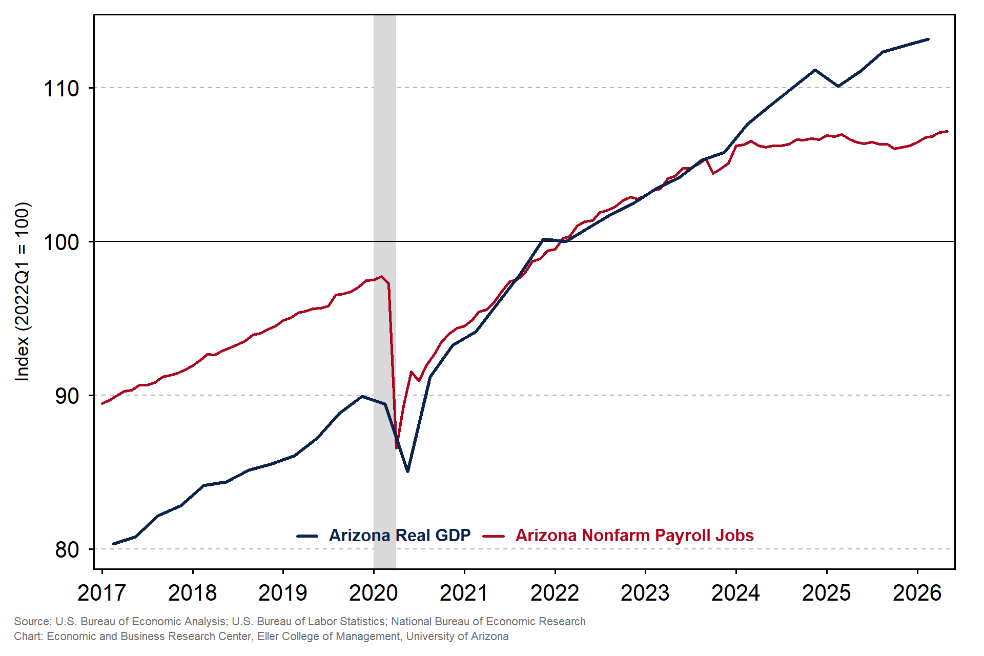
Like national data, Arizona’s real GDP has continued to grow despite little job growth since 2023, as shown in Exhibit 2. Real GDP recovered more strongly than nonfarm payroll employment after the pandemic, and the gap widened further as employment growth stalled while output continued to expand.
Exhibit 2: Indexes of Arizona Real GDP, Nonfarm Payroll Jobs, and Household Employment, First Quarter 2022 Equals 100
As signals from employment and output become more different, it is a good time to remind ourselves what GDP does and does not measure and how it is constructed at the national and regional levels. In theory, GDP can be constructed using the expenditure approach, the income approach, and the value-added approach. The three approaches yield the same total, because every dollar of value added (a producer’s sales minus its input costs) is a dollar someone spends on final output, and also a dollar of income to someone else. GDP releases from the Bureau of Economic Analysis (BEA) include both nominal and real numbers: nominal GDP measures output at the prices actually charged that year, while real GDP adjusts for inflation. Because real GDP strips out price changes, growth from one year to the next reflects more output, not more expensive output.
At any geographic level, GDP can tell us how the value of economic output is changing. However, different geographic levels offer different ways to understand contributions to overall economic output. In practice, only national GDP is built from all three approaches by the BEA, while the state and county GDP estimates rely primarily on the value-added and income approaches due to data limitations.[1]
National GDP is often discussed using the expenditure approach via the formula:
GDP = Consumption + Investment + Government Spending + Net Exports.
Consumption is household spending on goods and services, from groceries to rent to health care. Investment includes business capital spending (structures, equipment, and software) and residential construction. Government spending is what federal, state, and local governments purchase, while excluding transfer payments like Social Security. Net exports are what we sell abroad minus what we buy from abroad, to avoid double counting in consumption and investment. The breakdown for real U.S. GDP from 2025Q1 to 2026 Q1 in Exhibit 3 shows that consumption is consistently the largest component of output (~70%), and that investment and government spending combined make up about 35% of GDP, leaving a small negative share for net exports. This approach tells us how each expenditure type contributes to economic activity, but not how income is distributed across workers and firms or which industries produce the output.
Exhibit 3: Expenditure Components of Real U.S. GDP, 2025 Q1 to 2026 Q1, Percent of Total GDP
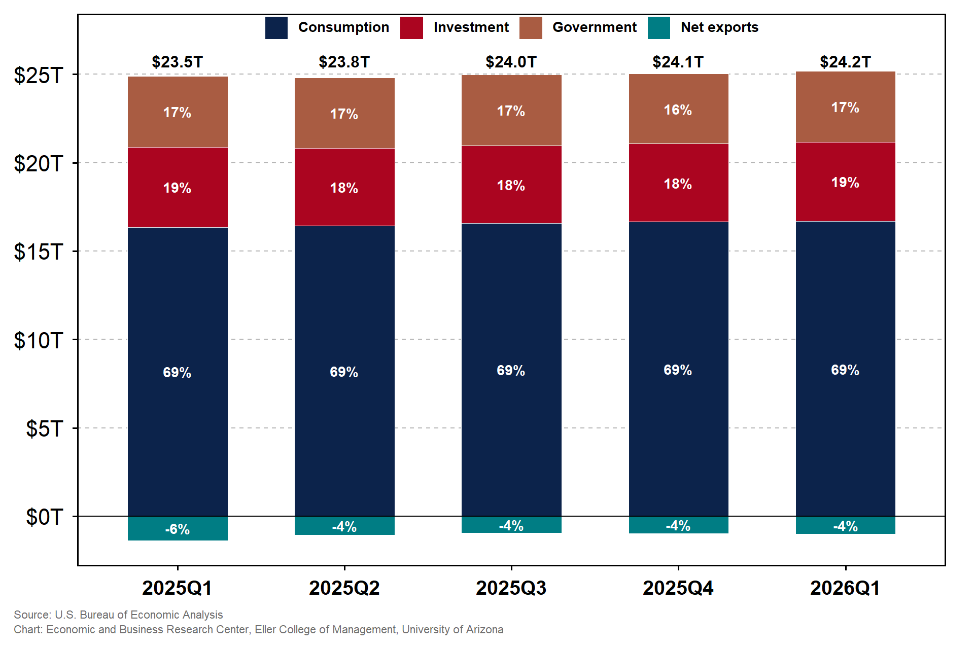
Note: A tiny reconciling residual (from BEA’s chain-weighting methodology, under which real GDP’s components don’t sum exactly to the total) is included in each bar but too small to see.
The value-added approach measures output for an industry as its sales minus the cost of the intermediate inputs (goods and services it buys from other businesses); subtracting the intermediate inputs prevents double counting along the supply chain. However, data to estimate sales and the cost of intermediate inputs at the state and local level are not available. Being the most geographically flexible of the three, the value-added approach organizes the economy industry by industry at all levels of BEA’s GDP releases, whereas the expenditure breakdown and the detailed income components largely stop at the national level.
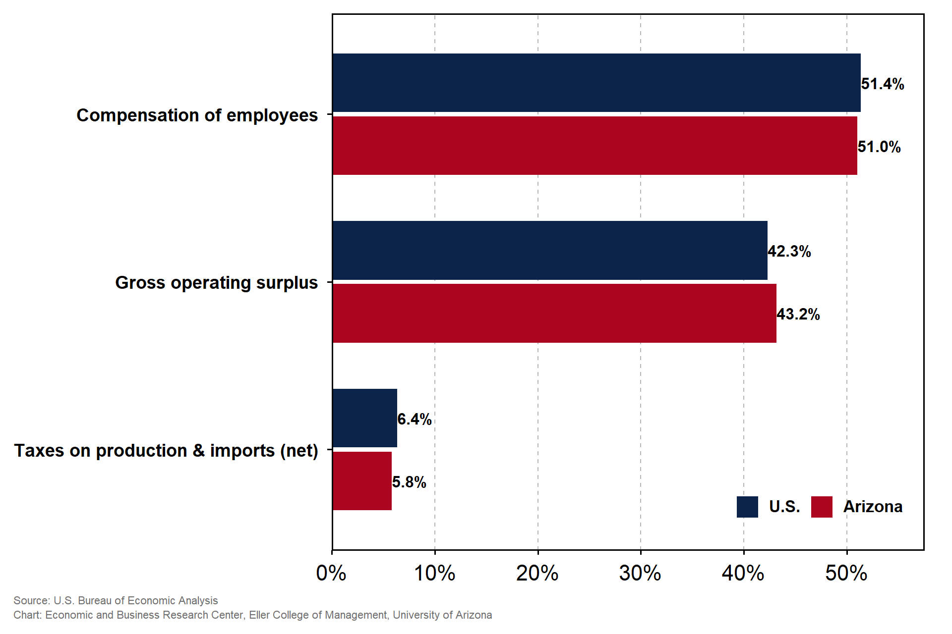
A third method to estimate GDP is the income approach, which sums income accruing to three factors of production: labor, capital, and government. Thus, the BEA adds up employee compensation, gross operating surplus, and net taxes of production and imports within a region. Exhibit 4 shows that in 2024, compensation of employees, which includes wages and employer-paid benefits, made up more than half of real GDP for both the U.S. and Arizona. Gross operating surplus, which is more than 40% of national income yet still smaller than employee compensation, sums up consumption of fixed capital (depreciation), corporate profits, proprietors’ income, rental income, and net interest and miscellaneous payments. Net taxes of production and imports capture tax payments to the government net of subsidies.
Exhibit 4: Income Components of Real U.S. and Arizona GDP, 2024, Percent of Total GDP
As labor force and GDP dynamics evolve with the changing demographics and technology landscape, it is increasingly important to understand what GDP can and cannot tell us. This is the first in a series of GDP explainers; the next will focus on Arizona’s economy and dig into the main income components and industries contributing to growth.
Extended Readings:
FRBB: Understanding the “Job-Loss Recovery”
FRBSF: Is Optimism for Artificial Intelligence Boosting Investment?
FRBSF: Have We Entered an Era of High Productivity Growth?
The Budget Lab: An AI Productivity Boom? Don’t Count Your (Productivity Data) Chickens
Working paper: The Broken Ladder: AI, Remote Work, and Early-Career Hiring
[1] The national GDP numbers are estimated by the BEA three times for each quarter, while the state numbers are estimated only once per quarter and released with the final national release. State GDP is value added by concept but also estimated through the income approach: output from goods-producing industries come directly from value-added production data, while output from services-producing industries is summed up from income components. For more details, please see https://www.bea.gov/resources/learning-center/what-to-know-gdp and https://www.bea.gov/resources/methodologies/gdp-by-state.