by George W. Hammond, EBRC director and Eller research professor
Nations, states, and local areas that concentrate on just a few industries are perceived to be riskier than more balanced regions. This makes good common sense. If we depend on one or a few sectors for most of our economic activity, then economic difficulty in those sectors will have a big impact on the aggregate economy.
Based on this reasoning, it is common for policy makers to suggest that diversification of the economy should be one important goal of economic development. While that is a very reasonable sentiment, it can be difficult to measure and implement.
For instance, what exactly do we mean by diversification? Does it mean that each industry should have an equal share of activity in the local economy? That does not seem to make much sense as an economic development goal.
Alternatively, local diversification could be measured relative to the U.S. In this case, a state or local area would be considered diversified if industry shares of local activity are close to the national average. This form of diversification would tend to make the local area about as risky as the nation.
Other measures of diversity borrow directly from the finance literature and focus on portfolio variance. The idea here is to imagine that the industries in a region are like securities held in a financial portfolio. Each industry has certain risk characteristics (variances, as well as covariances with other industries) that can be measured. Then the mix of industries could (theoretically) be adjusted to minimize risk for a given target growth rate. Pushing the finance analogy too far is problematic, however, because we cannot increase or decrease local industry activity with the same freedom that a portfolio manager can buy and sell securities.
An additional issue is the concept of economic activity. There are many measures of economic activity, each with its own strengths and weaknesses. Should we use employment, Gross Domestic Product, or income? In the literature, it is common to use employment, because that data is usually available consistently for long periods of time for all relevant geographies at a high level of industrial detail. Keep in mind, however, that the results can differ across concepts.
Classification details also matter. Most often, research into economic diversification uses NAICS industries. The results using NAICS industries will differ depending on the amount of detail used. For instance, an analysis using NAICS supersectors will differ from one using NAICS three-digit detail. Further, NAICS industries are only one way to conceive an “Industry.” After all, the “tourism” sector spans many NAICS industries. So does the “real estate” sector.
Finally, most of the research in the literature concludes that more diversified economies are more stable in the short run. In other words, they tend to have less dramatic short-run deviations from trend. There is less evidence that more diversified regions tend to grow faster in the long run.
Let’s take a look at one popular measure of diversification shows us about Arizona, the Phoenix Metropolitan Statistical Area (MSA), and the Tucson MSA. We will use the Hachman Index (developed by Frank Hachman at the University of Utah) to examine trends in employment diversification relative to the U.S. The index is defined as the reciprocal of the sum of industry-weighted location quotients, relative to the U.S. Expressed mathematically, for Arizona, that is:
Arizona Hachman Index = 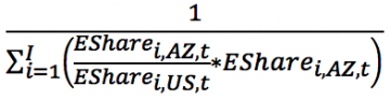 ,
,
where i indexes industries and EShare is the industry share of total employment. The ratio of the Arizona employment share to the national employment share is known as an Arizona location quotient. The Hachman index ranges from 1.0 (the region has the same employment mix as the U.S.) to 0.0 (the region has an employment mix as different as possible from the U.S.).
Just to put things in perspective, recent research using employment-based Hachman Indexes for states found that in 2014 they ranged from 0.98 (for Missouri) to 0.32 (for Wyoming).
Exhibit 1 shows Hachman Indexes for Arizona, the Phoenix MSA, and the Tucson MSA. The indexes were computed using employment data from the Current Employment Statistics program from 1990 to 2018 and 11 NAICS supersectors.
Exhibit 1: Arizona, Phoenix, and Tucson Hachman Index Trends, U.S. Recessions Shaded
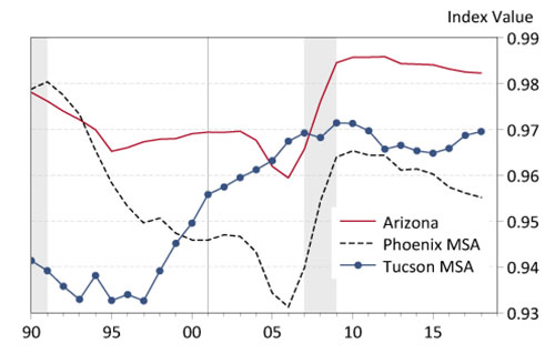
Note first that all three indexes are close to 1.0, indicating that at this level of industrial detail, employment mixes are similar to the nation. Indeed, the 2018 Arizona index value was 0.982, followed by 0.969 for the Tucson MSA, and 0.955 for the Phoenix MSA.
For Arizona and Phoenix the index declined through much of the 1990s and hit bottom in 2006. That indicated a gradual decline in diversity. During the Great Recession these indexes increased and then began to gradually decline during the recovery.
Tucson experienced a much different trend, with the index stable through the mid-1990s before beginning a gradual and sustained upward trend until just after the Great Recession, when it stabilized.
One advantage of the Hachman Index is that we can easily see what drove the trends. Exhibit 2 shows the sectors driving the change in the Arizona Hachman Index from 2006 to 2018. If we add all of the weighted location quotients for 2006 and then take the reciprocal, we get the Hachman Index for 2006.
Exhibit 2: Decomposing the Hachman Index for Arizona
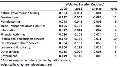
Note from the table that an increase in a weighted location quotient makes the Hachman Index smaller, indicating less diversification. A decrease in a weighted location quotient makes the Hachman Index larger, indicating more diversification. In this context, more diversification means an employment mix closer to the national average.
As Exhibit 2 shows, the weighted location quotient for education and health services increased the most from 2006 to 2018. That means that the industry share of employment in Arizona rose faster than the national average. Financial activities and leisure and hospitality made the next most important contributions. All three contributed to reduced diversification.
In contrast, construction posted the largest decline from 2006 to 2018, followed by professional and business services and government. Those declines contributed to increased diversification of the state employment mix.
Clearly, the biggest changes in employment mix in Arizona, relative to the U.S., occurred in construction and education and health services.
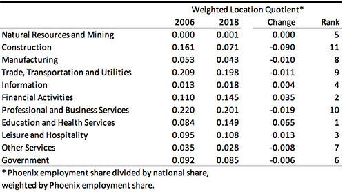
Exhibit 3 shows how the weighted location quotients evolved in the Phoenix MSA from 2006 to 2018. Similar to the state, the biggest changes were in construction and education and health services.
Exhibit 3: Decomposing the Hachman Index for the Phoenix MSA
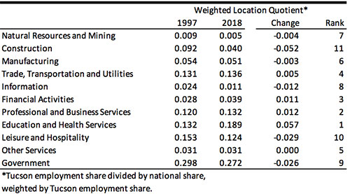
The Tucson Hachman Index differs from the state and Phoenix in that it shows a fairly strong upward trend during the past 21 years. What contributed to this? From 1990 to 2018, the largest contributions to increased diversification in Tucson came from construction; leisure and hospitality; and government (Exhibit 4). The largest contributions to decreased diversification came from education and health services; professional and business services; and financial activities.
Exhibit 4: Decomposing the Hachman Index for the Tucson MSA